Abstract
Concentrations of nitrogen (N), phosphorus (P), chlorophyll a (Chla), and dissolved oxygen (DO) were analyzed before and after the impact of six tropical cyclones (TCs) to determine their influence upon dead zones in the Chesapeake Bay. Using the Chesapeake Bay Data Hub, data was collected and analyzed using paired t test, both temporally and spatially. Temporally, TC Barry initiated the majority of the largest differences in concentrations with a decrease in DO (-1.51885 mg/L) and in Chla (-4.29649 µg/L). These drastic changes could be contributed to the time and track of Barry, and status of the Chesapeake Bay upon impact. All TC concentrations for each variable were averaged together to analyze spatial trends. DO concentrations increased throughout the Chesapeake Bay (0.903207 mg/L, 0.911879 mg/L, and 0.668812 mg/L) and were attributed to increased flow from tributaries. Examination of individual bay stations revealed the middle region of the bay is DO deprived and is a historically reoccurring dead zone. Both N and P concentrations decreased as latitude decreased and was contributed to the influx of salinity from the Atlantic Ocean. N concentrations were not significant either temporally or spatially leading to believe that P is the more limiting nutrient. It was concluded that future studies should include TC characteristics, salinity, and tributary data into the analysis of dead zones. The middle area of the bay should also be focused upon since it exhibits the greatest change in concentration. Understanding the influence of TCs upon dead zones can help better understand the health of the United States’ largest estuary.
Keywords: Tropical cyclone, dead zone, Chesapeake Bay
Introduction
Dead Zones in the Chesapeake
Each year water bodies worldwide are threatened by events so disastrous that they have been given the name “dead zones”. Dead zones have become an increasing concern globally as the number of dead zones has doubled each decade since the 1960s. Over 400 marine systems are affected by dead zones, covering an area of approximately 245,000 km2 (Diaz and Rosenberg 2008). The United States is home to two well-documented dead zones. The first is in the Gulf of Mexico at the outflow of the Mississippi River, and is the largest anthropogenic dead zone in the western hemisphere (Joyce 2000) and second largest in the world (Rabalais et al. 2002). The area of the gulf that is threatened each year is home to a $3 billion fishing industry and 40,000 related jobs, making dead zones catastrophic to the local economy (Malakoff 1998). This work will focus on a second major U.S. dead zone, located in the largest estuary in the world, the Chesapeake Bay. The Chesapeake Bay extends 200 mi from the Susquehanna River to the Atlantic Ocean. As a major fishery and tourism source, the Chesapeake Bay is a source of economic revenue for much of Virginia and Maryland.
Scientists attribute the increase of anthropogenic dead zones in the Chesapeake Bay to a chain reaction that begins with land use in the watershed. Agricultural and urban development has increased polluted runoff in coastal watersheds since the 18th century (Boesch et al. 2001). Due to the mismanagement of crop and animal agricultural practices throughout its watershed, the Chesapeake Bay and its tributaries suffer regularly from nutrient pollution or eutrophication (Diaz and Rosenberg 2008). Eutrophication in the Chesapeake Bay is estimated to have occurred as early as 250–300 years ago with the most rapid increase beginning around the 1940s (Cooper and Brush 1993). Most notably, the estuaries have experienced a substantial increase in nitrogen (N) and phosphorous (P). This is happening at a very large scale globally, and Vitousek et al. (1997) note that anthropogenic changes to the N cycle are double that of the carbon cycle.
Since N and P are essential nutrients for living organisms, when they exist in excess they support an exorbitant growth of aquatic biomass in the form of phytoplankton blooms. Such algal blooms occur naturally in the warm season, when there is ample light and an influx of new nutrients into a water body (Malone et al. 1988). Algal blooms are necessary for the Chesapeake Bay because phytoplankton are the dominant primary producers of the estuarine ecosystem (Joint and Pomeroy 1981) but they are known to have ramifications for habitats, ecosystems, and higher trophic levels (Paerl et al. 2007).
The algae flourish in the nutrient-rich waters. When they later die, they sink to the bottom where they are consumed by benthic organisms (Mee 2006). Bacteria work to decompose the algae and use oxygen in order to perform respiration. When the dissolved oxygen (DO) concentration falls below 2ppm or 2ml O2/liter, hypoxia is established and the water struggles to support marine life (Wenner et al. 2009, Diaz and Rosenberg 2008). Sometimes the water becomes completely devoid of DO (anoxic), especially in the bottom waters (Diaz 2001). Anoxia has been documented during the early and late summer in the Chesapeake Bay (Murphy and Kemp 2011). In the United States alone, hypoxia occurs naturally in half of the estuaries and anoxia occurs in about one third (Joyce 2000). Anthropogenic, and climatic factors, in addition to basin stratification, can often influence the occurrence of hypoxia, eutrophication, and algal blooms. With the increase of N-based fertilizers in the 1940s, there has been a notable decline of DO concentrations in many water bodies (Diaz et al. 2008).
The Impact of Tropical Cyclones
A dead zone forms in a body of water in part from an influx nutrients, namely N and P. Since 1945, the Chesapeake Bay has shown a significant increase of phytoplankton due to the input of nutrients from its tributaries (Jickells 1998). Thus, climatic events may flush excess nutrients to these waters, potentially spurring an algal bloom. Tropical cyclones (TCs) are believed to cause algal blooms and dead zones due to their ability to wash polluted runoff into the tributaries that feed the bay (Miller et al. 2006), and by mixing nutrients from the bottom waters (Wetz and Paerl 2008). As hurricane season is most active during the summer, algal growth is able to persist due to the plethora of light.
TC-induced dead zones have been documented in multiple water bodies. After Hurricane Floyd, Pamlico Sound of North Carolina suffered an algal bloom with an increase of chlorophyll a (Chla) from an average of 5-12 µ1-1 to 23 µ1-1 (Mallin and Corbett 2006). Between 1996 and 1999, Hurricanes Fran, Bonnie, and Floyd dramatically amplified the runoff of the Cape Fear River system and planktonic algae respirations were ten to fifty times greater (Mallin et al. 2002). In the Chesapeake Bay, Hurricane Isabel is documented as causing an abnormally large bloom by destratifying the bay and mixing the nutrients from the bottom waters. Flights conducted before and after Isabel showed a two-fold increase of Chla, covering an area of 3000 km. The bay returned to the long-term average by early October, one month after the hurricane’s passing (Miller et al. 2006).
Wetz and Paerl (2008) note that the likelihood of a TC inducing a dead zone depends mostly on the current status of the bay. For example, as in Hurricane Isabel’s case, if the bay is stratified then the TC may cause mixing of nutrients and increase the likelihood of a dead zone. Or, if the bay is lacking enough N (as N is usually the limiting factor in phytoplankton growth), the eutrophied runoff throughout the watershed may provide the N needed to spur algae growth. There have been scenarios in which a water body was deemed “dead” before a TC impact. An abnormally wet spring in 2011 caused an unusually large amount of polluted discharge to enter the Chesapeake Bay from its tributaries, and by early June a record 33% of the bay’s volume was deemed hypoxic. This climbed to 40% by July. That September, Hurricane Irene crossed the bay, mixing the waters and giving it a breath of oxygen. While her impact may have been momentarily positive, it is likely that her nutrient pollution has impacted the bay’s health negatively for the 2012 warm season (Maryland Department of Natural Resources).
The Significance of this Research
While research suggests that certain TCs are responsible past Chesapeake Bay dead zones, many of the studies are not easily repeated and therefore results are difficult to compare. For example, Miller et al. (2006) required extensive preparation and data collection prior to, during, and after the hurricane using aircraft surveillance and remote sensing equipment. While they provide a helpful perspective on the Hurricane Isabel algal bloom, this technique may only be used in rare circumstances. Klemas (2012) mentioned two studies that were cost beneficial in measuring Chla since satellite imaging was used, but this still requires extensive training in remote sensing techniques. It is the goal of this study to analyze Chesapeake Bay dead zones utilizing readily available water quality data and repeatable methodology.
In this study, concentrations of N, P, DO, and Chla are evaluated before and after recent TCs in the Chesapeake Bay. Individual TCs are analyzed to abserve their influence on bay nutrient levels, and the spatial differences in impacts across the bay. This information could provide greater insight on how dead zones are influenced by climatic factors such as TCs.
The TCs used in this study vary in size, direction of approach, and intensity, but as Wetz and Pearl (2008) noted, the characteristics of the TC should not matter significantly. The TCs that were selected have occurred within the past 10 years and have tracked within 160 kilometers of a central point in the bay (Figure 1). This distance was chosen because this is the distance Hurricane Isabel passed by the bay, which is reported to have caused a large bloom. The selected TCs are: Isabel (2003), Charley (2004), Gaston (2004), Ernesto (2006), Barry (2007) and Hannah (2008) (Table 1). Including Isabel will help compare this study to past results. Gaston and Charley, both 2004, will provide insight on the impact of multiple TCs in a row in the Chesapeake Bay, similar to how Gustav and Ike (2008) combined to create devastating effects to Louisiana’s marine ecosystems (Galvin et al. 2012). Data was analyzed one month before the TC passed through and one month after it passed. Wetz and Paerl (2008) show that the largest impacts of TCs on algal blooms are evident within a short time period after the TCs passing, and Miller et al. (2006) show that the bay recovered from the Isabel bloom within one month of the hurricane’s passing.
Previous research suggests that TCs have an impact upon Chesapeake Bay nutrient fluxes and dead zones. Water quality data collected by the Chesapeake Bay Data Hub has not been used extensively to study the impact of TCs on bay nutrient levels. The following research questions (Q1, Q2, and Q3) and hypotheses (H1, H2, and H3) are tested using the data.
Q1. Do the water quality data suggest that Chesapeake Bay TCs cause an increase of N and P in the estuary?
H01: There will be no significant differences in N and P amounts in the Chesapeake Bay before and after the TCs.
Q2. Do the water quality data suggest that Chesapeake Bay TCs cause an algal bloom?
H02: There will be no significant differences in in Chla and DO amounts in the Chesapeake Bay before and after the TCs.
Q3. Are the upper, middle, and lower parts of the bay affected differently by Chesapeake Bay TCs?
H03: There will be no significant differences between the three areas of the Chesapeake Bay before and after the TCs.
Data Collection and Methods
The water quality data utilized are from the Chesapeake Data Program database, available at (www.chesapeakebay.net/data), which extends from 1984 to the present. The database is a cooperation between the local, state, and federal government and contains data from 49 stations positioned throughout the bay and its watershed. For most of the variables, data is collected weekly during the warmer months and once a month during late fall and winter.
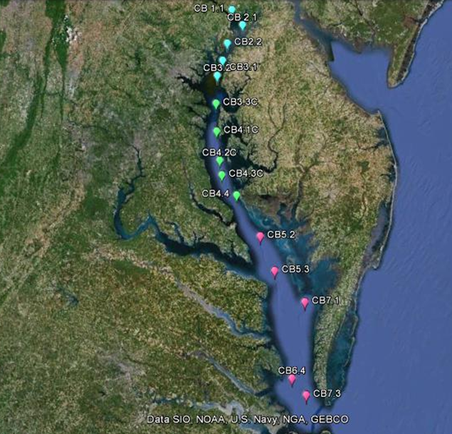
For this study, data are gathered from 15 pumping stations spread throughout the Chesapeake Bay (Figure 2). The stations were chosen primarily by data availability through the time period. Their location was also taken into account in order to have relatively even coverage across the estuary. The stations are grouped based on their location in the bay, each station being classified as “upper”, “middle”, or “lower” for the purpose of testing for spatial differences in TC impacts.
The variables collected for stations are N, P, Chla, and DO. The variables, N and P were collected in mg/L and Chla in µg/L. Nutrient variables, N and P, were collected in the form of total nutrients present within the bay to include both inorganic and organic. These measurements were analyzed in order to include all nutrients accessible for phytoplankton growth and availability of data. The nutrients (N and P) as well as Chla concentrations are collected at the surface and bottom of the water and possibly at two additional depths if there is a present pycnocline. In the presence of a pycnocline, nutrient measurements are collected at 1.5m above and 1.5m below the pycnocline depth. Otherwise, measurements are taken from the top and bottom layers of the water column. Unlike freshwater stations, predetermined depths are not effective for the bay since stratification can occur rapidly throughout the year. DO is measured in mg/L and is collected at approximately 1–2 m intervals. All collected data were averaged for each individual station based upon date. Data is gathered for one-month pre and post TC. The exact dates of the observations vary between pumping stations, with each station having one or two observations each pre and post TC. The number of observations is shown in Table 2.
Paired sample t-tests are used to test the hypotheses using the data collected. For Q1 and Q2, the four variables are tested for significant differences pre and post each TC. For Q3, the four variables are tested for significant differences in each location group pre and post TC, based on the average of all TC interceptions. The next section outlines the results of the t-tests, followed by a discussion of any notable results.
Results
Individual TC impacts
Table 3 displays the differences in mean concentrations across time pre and post TC, with bold numbers meaning there was a significant difference according to the paired sample t-test. The concentration with the most significant changes was DO, with half of the TCs causing a significant increase in DO. Only two TCs had a statistically significant impact on the concentrations of Chla (Isabel and Barry). The only concentration to not exhibit any significant differences between pre and post averages was N. Changes in P were also small but two TC’s were statistically significant (Isabel and Ernesto).
As measured by the data hubs distributed throughout the Chesapeake Bay, all TCs, except for Charley, had a significant impact on at least one concentration. Hurricane Isabel significantly impacted DO, Chla, and P but in the opposite manner of which I hypothesized, with an increase in DO (1.7605 mg/L) and decreases in Chla (-2.0459 µg/L) and P (-0.01086 mg/L). Barry initiated the majority of the largest differences in concentrations, including a significant decrease in DO (-1.51885 mg/L), making Barry the only TC that did not cause a positive change in DO concentrations.
Two TCs impacted the bay in 2004, so both were used to analyze the impact of two storms in one season. Charley, the first bay TC from 2004, had less of an impact than Gaston, the second TC of the season. The only significant change brought by either of the TCs was the increase in DO (1.86056 mg/L) caused by Gaston. DO (1.30413 mg/L) was also the only significant change brought by Hanna in 2008.
Spatial variability of TC impacts
Similar to the individual TC results, DO was the concentration most impacted by each part of the bay, with all parts of the bay showing a significant increase post TC (Table 4). N was not found to be significant in any areas of the bay upon analysis. The middle area of the bay experienced the most significant changes in concentrations, and exhibited a notable decrease in Chla (-2.77673 µg/L) post TC.
The data for each concentration are plotted from north to south in Figures 3-6 in order to show the spatial patterns in concentrations and fluxes. N concentrations decreased overall with latitude. The highest recorded N concentration was post TC for CB1.1 (1.5301 mg/L) and the lowest average nitrogen concentration was station CB7.3 pre TC (0.345419 mg/L). There were no significant differences pre and post TC. P was also found to have a decreasing trend towards the more southern end of the bay. CB5.3 had an abnormal high P reading post TC at 0.22143 mg/L, perhaps an erroneous reading. Chla concentrations showed no remarkable spatial pattern, with the highest increase at station CB3.3C (12.191 µg/L) pre TC. Additionally, dissolved oxygen was significant in all areas of the bay between pre and post averages. DO concentrations decreased and increased in a parabolic fashion from north to south of the bay, with the middle of the bay having the lowest DO readings. The lowest recorded DO concentration was CB4.1C (2.716421 mg/L) pre TC and the highest was CB2.1 (8.004821 mg/L) post TC.
Discussion
Individual TC Impacts
It was expected that TCs would cause an increase in nutrients N and P due to eutrophication of tributaries and mixing of the bay’s water. This could result in an algal bloom, which would be signified by a substantial increase in Chla and a decrease in DO. The results reveal an opposite trend than anticipated in most of the variables and TCs.
N concentrations were expected to increase due to eutrophication and destratification. Algal blooms can occur due to eutrophication of the bay since N is often a limiting factor in oceanic, coastal, and estuarine waters (Paerl 1997). It was expected for N to increase during the impact of Isabel since there was a large algal bloom and vertical mixing of the water columns. The results presented no significant changes in N for any of the TCs. Besides dilution of the nutrient in the bay, other factors outside the bay may also contribute to the decrease, including soil absorption, plant uptake, microbial uptake, and denitrification of standing nutrient-rich waters on flood plains (Mallin et al. 2006). Inability to fully examine tributary variables may have led to a misunderstanding of the cause of N concentration during the TCs.
Comparatively, P concentrations were also expected to increase after TC tracks due to expected eutrophication of the bay by potential runoff from tributaries. However, the only two TCs to demonstrate any significant differences were Isabel (-0.01086) and Ernesto (-0.01885) in which P decreased (Table 3). A comparison of two consecutive hurricane seasons in the Neuse River Estuary and Palmico sound revealed shallow estuaries are able to recover from frequent hurricane impacts in regards to high nutrient loads of N and P (Burkholder et al. 2004). Data analyzed after TC impacts was limited due to insufficient consecutive collection of data after TC impacts. Similar to N concentrations, dilution may have also played a factor in decreased P concentrations as well. Glasgow and Burkholder (2000) found that P decreased as high volumes of flow entered the Neuse River Estuary between two consecutive years. This could be a possible explanation to why P overall decreased but could not be measured due to lack of tributary data.
After eutrophication it was expected to see an increase in Chla and decrease in DO, signifying a dead zone. Once again the data showed the opposite of what was expected. A specific example is Hurricane Isabel; where previous studies presented a decrease in DO due to the large algal bloom that resulted from winds of Isabel destratifying the bay’s water column by vertical mixing (Li et al. 2006). This should be evident through an increase in Chla concentrations. Miller et al. (2005) found 6 days after Isabel, Chla increased spatially two to three times the long term average. With such a large algal bloom, it would then be expected that a dead zone would result and be evident in the DO concentrations. However, the water quality data show a decrease in Chla and increase in DO, not supporting these ideas. One possible reason could be that Miller et al. (2005) are only seeing a spatial spreading of the algal bloom, rather than an actual growth of additional algae. From an aircraft the expanded algal bloom could resemble a growing bloom rather than one that has been mixed across the surface. This would cause a decrease in Chla concentrations at an individual station. The turbulent mixing of the waters could also favor an increase in DO in the readings, similar to the Irene example discussed in the introduction.
Gaston and Charley were selected to study the effects of two consecutive TCs upon the bay. Based upon the data, successive TCs were inversely related to each other except in DO concentration (Table 3). Gaston only had one significant difference in DO (1.86056) while Charley had no significant differences. Peierls et al. (2003) discovered that variable Chla and N and P can be inversely related to each other during the occurrence of consecutive TCs. Based upon the Peierls et al. (2003) study, it is plausible that an algal bloom occurred during Charley (increase in Chla) that lead to the usage of N and P by the phytoplankton for growth (decrease in N and P). When Gaston then hit only a short time after, the increase of N and P could have been attributed to a flux of nutrients from rivers. The decrease of Chla may be due to increase of turbidity by Gaston, which would limit light for phytoplankton for growth.
Spatial Variability of TC Impacts
Spatial variability of TC impacts were studied to determine differences in concentrations among the bay areas, as well as differences in their response to TCs. Both N (Figure 3) and P (Figure 4) gradually decrease with a decrease in latitude. In areas of the Chesapeake Bay where salinity is typically lower, N and P concentrations were found to be higher (Boynton et al. 1995). Smith (1984) also presented that as salinity increased, P inversely decreased, while N typically remained the same. This trend is noticeable, as the lower latitude stations have decreased concentrations of N and P compared to that of the middle and upper bay. Being closer to the mouth of the bay allows water from the Atlantic Ocean to enter and gives the lower stations higher salinity levels (Chesapeake Bay Foundation).
After the TCs passed, the lower part of the bay showed no significant changes in nutrient concentrations. The upper and middle bay areas reported a significant change in P, although inversely from one another (decreasing in the upper area and increasing in the middle area). None of the areas were significantly impacted by N. Paerl et al. (2006) discovered factors such as water residence time and stratification could play a role in nutrient concentrations. As water stands in areas such as flood plains, nutrients, such as N and P, are gradually leeched and used by biological processes. This process then decreases the amount of nutrients in the bay.
There were no obvious spatial patterns in Chla based on location in the bay. The only area determined to have any significant difference of Chla concentration from TC passage was the middle bay (Table 4), which showed a decrease in concentrations (Figure 5). This was unexpected since it was thought that TCs would cause an algal bloom due to eutrophication or destratification of the bay. Turbidity of tributary waters could have played a factor in Chla concentrations present within the bay. Irigoien and Castel (1997) found that the photosynthetic activity of Chla decreases with increases of water turbidity. It is possible that TCs generated enough flooding of tributaries that excess debris entered the bay, thus decreasing the concentration of Chla.
There is an obvious dip in DO in the middle of the bay, with the highest values being to the north and south (Figure 6). A comparable trend was found in a study where the north and south area of the bay had similar DO concentrations and the middle bay had significantly lower DO measurements. Cowan and Boynton (1996) accredited this trend to reduced vertical mixing and increased loading of organic matter in sediments. Reduced vertical mixing may have been contributed to the pycnoclines. The Chesapeake Bay Foundation reported that pycnoclines occur naturally in between the Potomac River and the Bay Bridge (Chesapeake Bay Foundation). This area was deemed the middle area in this project. Oxygen would not be able to penetrate through a pycnocline, where it would then turn into DO in bottom water columns. Kelly and Doering (1999) presented that DO concentrations vary horizontally within the Chesapeake Bay, as the pycnocline is influenced by wind-induced tilting and oscillating. An analysis of pynocline data before and after each TC could further explain these results.
DO increased significantly post TC for all three bay areas (Table 4). When the TCs made their way through Virginia, it is possible they were able to flush out more water into the bay and increased its flow. By increasing the flow of the bay, oxygen from the air is able to dissolve into the water, thus increasing DO concentrations (Chesapeake Bay Foundation). In future studies, quantifications of the flow of the bay pre and post TCs may contribute to the understanding of DO fluxes within the bay.
Conclusion
The purpose of this study was to investigate the influence of TCs upon nutrient fluxes and dead zones of the Chesapeake Bay using readily available data. Three research questions (Q1, Q2, Q3) were derived to investigate the following prospects: influence of TCs upon N and P influx within the bay, reliability of water quality data to predict an algal bloom, and possible spatial differences among the bay. The null hypotheses (H1, H2, H3) presented that there would be no changes to the bay due to TCs or water quality data would not reveal algal blooms. Data collected by the Chesapeake Bay Foundation were analyzed one-month prior and post TC impact. Data were collected from 15 stations located throughout the bay and analyzed independently for each TC and in spatial groupings using paired sample t-tests. The results demonstrate spatial trends of nutrients and nutrient fluxes within the bay. These specific trends did not support hypothesis and open an interesting discussion of how TCs affect the Chesapeake Bay, as well as the reliability of water quality data.
The hypothesized results of this study were that a TC would increase nutrients and eutrophication and a resulting increase of Chla and decrease of DO. This would cause a dead zone within the bay. It is interesting result that the algal bloom that reportedly occurred after Isabel was not evident in the water quality data. The way in which data was collected in past studies could have contributed to controversial Chla measurements such as that in Miller et al. (2005). Aerial data could record the growth of algal by satellite imaging, but possibly the concentration of Chla could be much lower due to spatial dispersion from the churned waters.
Furthermore, possible reasoning behind the DO trend witnessed in the data could be contributed to organic matter from previous years determining the overall DO concentration and not phytoplankton. Similarly, other TCs displayed erratic significant differences among their variables. It was decided that N and P are greatly influenced by biological tributary processes, which limit the flux of these variables into the bay. It was also determined that overflow from tributaries could have diluted N and P concentrations within the Chesapeake Bay after individual TCs.
Spatially, a trend was noticed in N and P as latitude decreases towards the southern end of the bay. The variable contributing to this trend was most notably salinity. As salinity increases, concentrations of N and P inversely decrease. The lower stations were closer to the mouth of the bay where salinity conditions are higher due to the Atlantic Ocean. Upon further evaluation of the spatial data, the biggest area to exhibit differences among variables was the middle portion. Reasoning behind why the middle bay differs greatly may be contributed to shape of the Chesapeake Bay’s bottom. Due to the similarity to a bowl shape, most notable in the middle area of the bay, pycnoclines can very easily act a lid and prevent the flow of oxygen to bottom layers (Chesapeake Bay Foundation). This could possibly explain why this area of the bay had such a tremendous decrease in DO compared to the other two areas. In addition, Chla was only found significant in this area of the bay as it decreased. Turbidity of waters could have played a factor in this concentration. For future studies, the middle area of the bay should be focused upon due to it s tendency to exhibit the greatest influence from TCs.
Previous studies argued about the importance of TC characteristics versus current status of the bay as being the predictor of a TCs impact. Intensity or track may not be a perfect predictor of impact due to influx of nutrients often being attributed to either mixing or runoff into tributaries. However, it is important to look at storm variables that may impact these two factors. I believe future studies should include TC characteristics (strength, track, speed, rain fall amounts, etc.) as they can greatly alter the bay’s composition through factors, such as dilution, and mixing of columns. That being said, the current status of the bay is also important. As seen in the results of this project, if the bay waters are already high in Chla or low in DO, a TC may impact the bay in the opposite way one would expect. As shown by Barry, if any levels are abnormally high the TC may help them reach their natural equilibrium. In the case of Barry, newspaper articles suggest that a dead zone was beginning to form, hence the high Chla concentration. It would be interesting in future studies to analyze the impact of Barry upon that potential dead zone. Further investigations of Barry could also reveal whether time of year was the cause for such differences when compared to the other TCs.
Data collected for the experiment were solely from the Chesapeake Bay Data hub. These open source data provide a more streamlined, inexpensive way to analyze bay health, compared to individual sampling methods, remote sensing, and other collection methods used in past studies. However, the data also come with a set of issues. First, the data lack temporal resolution and regularity. The data is only collected every couple of weeks, and still some stations were unable to provide numerical data pre and/or post TC. The stations used in this study were some of the few that had the data available for both time periods. This is still not ideal, as it is important to see the small scale changes in nutrient levels to understand TC impacts, which would require at least daily observations. If the data hub was able to provide a more extensive record of data collection, variables collected would have been more reliable statistically. Second, this study initially involved the study of the tributaries to determine the cause of eutrophication. However, due to sporadic data availability, especially in the most important bay tributaries (e.g. Susquehanna River), this was an impossible feat with these data.
Without fully understanding eutrophication, it could not be determined if N and P fluxes in the bay were being caused primarily by tributary or bay variables. Since the results differed rather substantially from a number of past studies, this research encourages further studies to analyze the impact of TCs on Chesapeake Bay nutrient levels. While the data would improve with increased spatial and temporal sampling, they are still data from 15 points in the bay that are signifying a different relationship that previously believed.
Lack of salinity data also led to a misunderstanding of N and P concentrations within the bay. It could not be determined if salinity was a major factor in N and P trends or a lack of tributary data. Salinity data in future studies could be used to show similarities compared to that N and P concentrations, which should be inversely related. In addition, a lack of pycnocline data could not fully establish whether DO data was influenced by flow of the bay or an inability of oxygen to penetrate to lower water columns. By incorporating these three factors into future research the DO, N, and P concentrations could be understood more fully, as well as the impacts of TCs on the health of the world’s largest estuary.
Acknowledgements
I am indebted for the constant support and guidance provided by my research advisor Dr. Kelsey Scheitlin as this project would not have been plausible without her. I greatly appreciate the use of the data and information provided by the Chesapeake Bay Data program in order to perform this study. I would like to thank my senior honor’s research examining committee for allotting a portion of their time for my defense presentation and providing feedback on my thesis. I am grateful to Dr. Kenneth Fortino for providing insight on the biogeochemical nature of nutrients used in this study. Lastly, I am obliged toward Longwood University in allowing me to perform this research.
Tables and Figures
| Name | Year | Month | Distance |
| Isabel | 2003 | 9 | 98 |
| Charley | 2004 | 8 | 62 |
| Gaston | 2004 | 8 | 49 |
| Ernesto | 2006 | 9 | 23 |
| Barry | 2007 | 6 | 94 |
| Hannah | 2008 | 9 | 13 |
Table 1: TCs that will be used in the study. Distance is their distance in miles from a central point in the Chesapeake Bay (mapped in Figure 2).
| Upper Bay Observations | Middle Bay Observations | Lower Bay Observations | |
| Isabel | 20 | 19 | 12 |
| Charley | 15 | 15 | 17 |
| Gaston | 15 | 15 | 16 |
| Ernesto | 15 | 15 | 13 |
| Barry | 20 | 17 | 15 |
| Hanna | 15 | 15 | 13 |
Table 2: Number of bay observations observed for each designated area per individual TC. Observations were averaged for each individual station for each date collected.
| N | P | Chla | DO | |||||||||
| Hurricane | Pre | Post | Change | Pre | Post | Change | Pre | Post | Change | Pre | Post | Change |
| Isabel | 0.922262 | 0.937216 | 0.01495 | 0.062826 | 0.051961 | -0.01086 | 8.167145 | 6.121266 | -2.0459 | 4.697332 | 6.457852 | 1.7605 |
| Charley | 0.866947 | 0.809619 | -0.05733 | 0.051836 | 0.050921 | -0.00091 | 6.061629 | 6.419151 | 0.35752 | 4.684345 | 5.346266 | 0.66192 |
| Gaston | 0.869117 | 0.937461 | 0.06834 | 0.055953 | 0.077246 | 0.02129 | 6.831968 | 4.513937 | -2.31803 | 5.253362 | 7.113922 | 1.86056 |
| Ernesto | 0.650388 | 0.75746 | 0.10707 | 0.063816 | 0.044967 | -0.01885 | 6.147159 | 6.271339 | 0.12418 | 4.569955 | 5.440371 | 0.87042 |
| Barry | 0.890848 | 0.757386 | -0.13346 | 0.032212 | 0.078796 | 0.04658 | 11.30365 | 7.007163 | -4.29649 | 6.656867 | 5.138022 | -1.51885 |
| Hanna | 0.630086 | 0.610686 | -0.0194 | 0.062344 | 0.055798 | -0.00655 | 8.14438 | 5.475898 | -2.66848 | 3.954823 | 5.258954 | 1.30413 |
Table 3: Averages of 15 selected bay stations per TC for each variable. Differences between pre and post TC concentrations based on the average of 15 selected bay stations. Bolded numerals indicate a significant (p<0.05) difference according to a paired-sample t-tests.
| Bay Area (stations) | Chla | DO | P | N |
| Upper (CB1.1 -CB3.2) | -1.93009 | 0.903207 | 0.014463 | 0.059687 |
| Middle (CB3.3C-CB4.4) | -2.77673 | 0.911879 | -0.01641 | 0.008966 |
| Lower (CB5.2-CB7.3) | 0.075108 | 0.668812 | 0.022043 | -0.00648 |
Table 4: Differences between pre and post TC concentrations in three segments of the bay (upper, middle, and lower). Bolded numerals indicate significant changes (p<0.05) in means according to paired sample t-tests.

Figure 1: Tracks of the TCs being used in the study. The darkest tracks passed nearest the black point in the Chesapeake Bay, while all passed within 100 mi. Hurricane Isabel, known to have caused an algae bloom in the Chesapeake Bay, is the light grey track that continues inland toward the Great Lakes.

Figure 2: Location of stations within the Chesapeake Bay (Courtesy of Google Earth Maps). Light blue pegs indicate upper bay stations, green pegs indicate middle bay stations, while pink pegs indicate lower bay stations.

Figure 3: Average N concentration for each station North to South along the Chesapeake Bay. The blue line is the pre-TC average and the red line is post-TC average.

Figure 4: Average P concentration for each station North to South along the Chesapeake Bay. The blue line is the pre-TC average and the red line is post-TC average.

Figure 5: Average Chla concentration for each station North to South along the Chesapeake Bay. The blue line is the pre-TC average and the red line is post-TC average.

Figure 6: Average DO concentration for each station North to South along the Chesapeake Bay. The blue line is the pre-TC average and the red line is post-TC average.
Literature Cited
About the Bay. [Internet] Chesapeake Bay Foundation [cited 2012 June 12] Available online at: http://www.cbf.org/about-the-bay
Boesch D, Burreson E, Dennison W, Houde E, Kemp M, Kennedy V, Newell R, Paynter L, Orth R, Ulanowicz R, Peterson C, Jackson J, Kirby M, Lenihan H, Bourque B, Bradbury R, Cooke R, Kidwell S. 2001. Factors in the decline of coastal ecosystems. Science. 293:1589–1591
Boynton WR, Garber JH, Summers R, Kemp WM. 1995. Inputs, transormations, and transport of nitrogen and phosphorus in Chesapeake Bay and selected tributaries. Estuaries. 18:285–314
Burkholder J, Eggleston D, Glasgow H, Brownie C, Reed R, Janowitz G, Posey M, Melia G, Kinder C, Corbett R, Toms D, Alphin T, Deamer N, Springer J. 2004. Comparative impacts of two major hurricane seasons on the Neuse River and western Pamlico Sound ecosystems. Proceedings of the National Academy of Sciences. 101(25):9291–9296
Cooper SR and Brush GS. 1993. A 2500-year history of anoxia and eutrophication in Chesapeake Bay. Estuaries. 16: 617–626
Cowan JLW and Boynton WR. 1996. Sediment-water oxygen and nutrient exchanges along the longitudinal axis of Chesapeake Bay: seasonal patterns, controlling factors and ecological significance. Estuaries. 19(3):562–580
Diaz RJ and Rosenberg R. 2008. Spreading dead zones and consequences for marine ecosystems. Science. 321:926–929
Diaz, R.J. 2001: Overview of hypoxia around the world. Journal of Environmental Quality. 30: 275–281
Galvin K, Bargu S, White JR, Li C, Sullivan M, Weeks E. 2012. The effects of two consecutive hurricanes on basal food resources in a shallow coastal lagoon in Louisiana. Journal of Coastal Research. 28:407–420
Glasgow HB and Burkholder JM. 2000. Water quality trends and management implications from a five-year study of a eutrophic estuary. Ecological Applications. 10(4):1024–1046
Irigoien X and Castel J. 1997. Light limitation and distribution of chlorophyll pigments in a highly turbid estuary: the Gironde (SW France). Estuarine, Coastal and Shelf Science. 44:507–517
Jickells TD. 1998. Nutrient biogeochemistry of the coastal zone. Science. 281:217–222
Joint IR and Pomeroy AJ. 1981. Primary production in a turbid estuary. Estuarine, Coastal and Shelf Science. 13: 303–316
Joyce S. 2000: The dead zones: Oxygen-starved coastal waters. Environ. Health. Perspec. 108:120–125
Kelly JR and Doering PH. 1999. Seasonal deepening of the pycnocline in a shallow shelf ecosystem and its influence on near-bottom dissolved oxygen. Marine Ecology Progress Series. 178:151–168
Klemas K. 2012. Remote sensing of algal blooms: an overview with case studies. Journal of Coastal Research. 28:34–43
Li M, Zhong L, Boicourt WC, Zhang S, Zhang D. 2006. Hurricane-induced storm surges, currents, and destratification in semi-enclosed bay. Geophysical Research Letters. 33:1–4
Malakoff D. Coastal Ecology: Death by suffocation in the Gulf of Mexico. Science. 281(5374):190–195
Mallin MA and Corbett CA. 2006. How hurricane attributes determine the extent of environmental effects: multiple hurricanes and different coastal systems. Estuaries and Coasts. 29:1046–1061
Mallin MA, Posey MH, McIver MR, Parsons DC, Ensign SH, Alphin TD. 2002. Impacts and recovery from multiple hurricanes in a piedmont-coastal plain river system. BioScience. 52:999–1010
Malone TC, Crocker LH, Pike SE, Wendler BW. 1988. Influences of river flow on the dynamics of phytoplankton production in a partially stratified estuary. Marine Ecology Progress Series. 48:235–249
Mee L. 2006. Reviving dead zones. Scientific American. 295:78–85
Miller WD, Harding LW, Adolf JE. 2005. The influence of Hurricane Isabel on Chesapeake Bay phytoplankton dynamics. Chesapeake Research Consortium. 160:155–160
Miller WD, Harding LW, Adolf JE. 2006. Hurricane Isabel generated an unusual fall bloom in Chesapeake Bay. Geophysical Research Letters. 33:1–4
Murphy RR and Kemp WM. 2011. Long-term trends in Chesapeake Bay seasonal hypoxia, stratification, and nutrient loading. Estuaries and Coasts. 34:1293–1309
Paerl HW. 1997. Coastal eutrophication and harmful algal blooms: Importance of atmospheric deposition and groundwater as “new” nitrogen and other nutrient sources. Limnology and Oceanography. 42:1154–1165
Paerl HW, Valdes LM, Peierls GL, Adolf JE, Harding LW. 2006. Anthropogenic and climatic influences on the eutrophication of large estuarine ecosystems. Limnology and Oceanography. 51:448–462
Paerl HW, Valdes LM, Joyner AR, Peierls BL, Piehler MF, Riggs SR, Christian RR, Eby LA, Crowder LB, Ramus JS, Clesceri EJ, Buzzelli CP, Luettich RA. 2006. Ecological response to hurricane events in the Pamlico Sound System, North Carolina, and implications for assessment and management in a regime of increased frequency. Estuaries and Coasts. 29:1033–1045
Paerl HW, Valdes-Weaver LM, Joyner AR, Winkelmann V. 2007. Phytoplankton indicators of ecological change in the eutrophying Pamlico Sound system, North Carolina. Ecological Applications. 17:88–101
Peierls BL, Christian RR, Paerl HW. 2003. Water quality and phytoplankton as indicators of hurricane impacts on large estuary ecosystem. Estuaries. 26(5):1329–1343
Rabalais NN, Turner RE, Wiseman WJ. 2002. Gulf of Mexico hypoxia, a.k.a. “The Dead Zone”. Annu. Rev. Ecol. Syst. 33:235–263.
Smith SV. 1984. Phosphorus versus nitrogen limitation in the marine environment. Limnology and Oceanography. 29(6):1149–1160
Update on the Chesapeake Bay summer dead zone (early August 2011). [Internet] Maryland Department of Natural Resources. [cited 2012 June 2]. Available online at: http://mddnr.chesapeakebay.net/eyesonthebay/stories/DOpredictionsAug2011_Update1.pdf
Vitousek PM, Aber JD, Howarth RW, Likens GE, Matson PA, Schindler DW, Schlesinger WH, Tilman DG. 1997. Human alteration of the global nitrogen cycle. Ecological Applications. 7:737–750
Wenner E, Sanger D, Arendt M, Holland AF, Cehn Y. 2009. Variability in dissolved oxygen and other water-quality variables within the national estuarine research reserve system. Journal of Coastal Research. 10045:17–38
Wetz MS and Paerl HW. 2008. Estuarine phytoplankton responses to hurricanes and tropical storms with different characteristics (trajectory, rainfall, winds). Estuaries and coasts. 31:419–429